Making a Computer Dream of New Jobs
A lot of things depend on how the labour market will change: whether we will have to get a new job, be paid more money or consider moving to a new city for work. Policy makers are particularly interested in job creation and all the benefits that this brings. This is very often discussed at the same time as technological change. Although many people assume that technology always takes jobs away, new technology has the potential to create new jobs. Taking the example of self-driving trucks, it’s likely that wages for truck drivers will reduce forcing many out of that job. But this has the potential to create both new high tech jobs, such as computer vision experts, and new jobs closer to the old ones, such as maintaining, designing and fixing the new self-driving trucks. Daron Acemoglu and Pascal Restrepo discuss this in detail.
The problem is that it’s very hard to predict which new jobs will be created. We don’t have good historical and structured data, we only have anecdotes to go on; the most famous of which is that Elevator Operator is the only occupation to totally disappear in the last few decades. Is there some way we can attack this problem and model what will happen without explicit data? As this short proof of concept notes, yes there is!

The first step is to think of a job as a set of tasks. A task is something that an organisation needs to be done like Managing Financial Resources or Withstanding Extreme Temperatures. The O*NET database from the Bureau of Labour Statistics in the US provides this based on interviews with workers, and they report a numerical weight for each task for each job. This gives us a job-task matrix.

Of course there is considerable structure in this matrix. There are certain tasks that are found together in many jobs. We can use this as a feature matrix and try to approximate the joint distribution of tasks in jobs. Based on this, we can then create new jobs as new samples from this distribution!
To do this, we need to build a generative model. This is a particular kind of machine learning model that creates new synthetic data based on some training data. We might also be able to prompt the data-generating process to produce new data that has certain characteristics. The most famous example of this is from image creation. One of the pioneers Alex Graves famously described generative models as having ‘machines that dream’; we want an algorithm that can dream up what a new job might look like.
There are two main generative models: Generative Adversarial Networks (GAN) and Variational Auto-encoders (VAE). These were introduced in papers by Ian Goodfellow and colleagues and Kingma and Welling respectively. Both models work quite differently, despite both producing new synthetic data based on training samples.
The GAN uses two modules, one to create samples and the other to try to classify the samples as synthetic or not. Once it has trained to the point that they cannot be distinguished with a certain accuracy, the model has converged. The VAE learns to compress the input data into a set of hidden nodes before decoding back to the full dimensionality of the data, hopefully in a loss-less way. The key part of the VAE is that it learns a distribution over the the hidden unit activations and thus the outputs are probabilistic. This has a regularising effect and also allows for a continuous and meaningful latent space to be constructed.
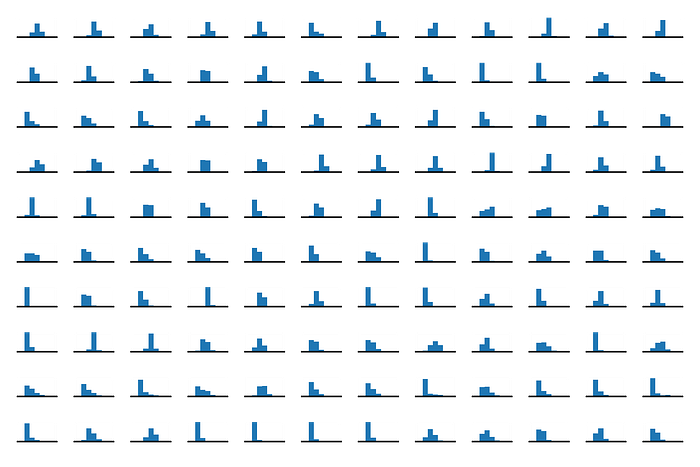
And each job is a distribution over these tasks. Take Desktop Publishers and Power Distributors and Dispatchers as examples (the full notebook is here).


You can see that the requirements of Desktop Publishers and Power distributors and dispatchers are different, but in many ways similar. In fact some skills are quite ubiquitous: they have a common value for all jobs because they are general. The tasks are evaluated for each job as the average of a set of survey responses on a scale 0–7. But as you can see, the distribution of each skill is far from the same

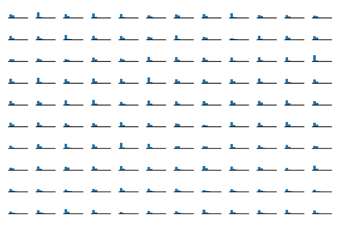
For that reason we apply a standard rescaling to the z-score.

After you do that, the two jobs start to look more distinct from each other.


In this case I borrow from Francois Chollet’s keras implementation of the VAE from his great book Deep Learning with Python. There are basically two components to the VAE; (i) the encoder layer that compresses the raw data into activations of a smaller number of latent dimensions and (ii) the decoder that samples from the latent activations and produces a vector of the same dimension as the original data. In order to make the reconstruction faithful, the original data and the encoded and then decoded output should be as close as possible.

In this case I chose a latent dimension of 4, which compresses from the original 120 task weights in each job and split the data into training and test data in the ratio roughly 90:10. The VA loss function has two parts; the first is a standard reconstruction loss which measures how far the original data and encoded/decoded data are apart. The second is a regularisation loss that forces the distribution over the latent units to be well behaved.

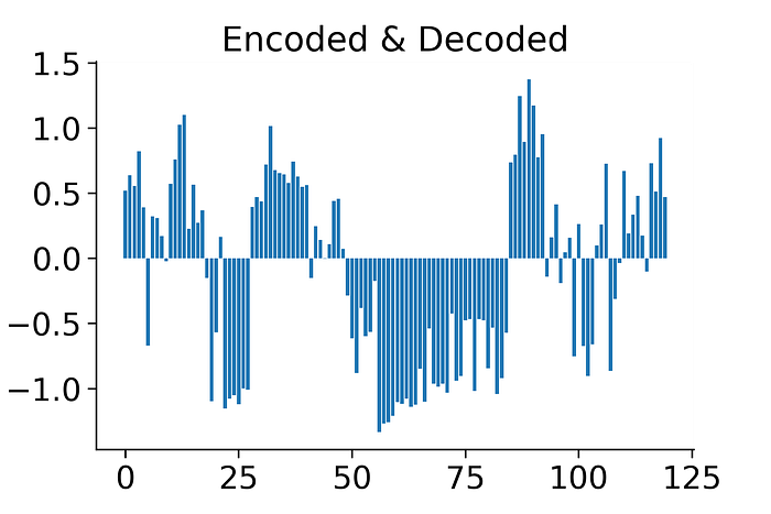
After 100 training epochs, the VAE reports a batch validation loss of 46.7. The VAE uses a loss function that is not only the reconstruction loss (how much information is lost between encoding and decoding) but also a term related to the prior distribution over the latent variables, related to the variational lower bound. This post does a great job in breaking down this loss function and the relation to a Bayesian interpretation. Consequently, this loss is a bit hard to interpret. As a sanity check, how does the VAE perform in encoding and decoding an arbitrary job?


From naive inspection, the distribution over tasks in the decoded output seems to match the input well, so the VAE seems to be picking up on the structure. The cosine distance between these two distributions is 0.067. It can be quite hard to interpret this accuracy! But we do know the distances between the original jobs in our data, we would hope that the distance between the input and output of our VAE should be much smaller with respect to the typical distance between jobs in our original data. Otherwise the VAE is spitting out something that bears less resemblance to the job that it is trying to compress, than do a pair of arbitrary jobs to each other.

Luckily, the distances between the (out of sample) inputs/outputs of the VAE are much smaller than the pairwise distances between the training data; a mean of roughly 0.24 vs 1.0.
Now the fun part begins! We can now artificially activate the latent dimensions that feed into the decoder. Now we can sweep through the parameter space of the latent states and generate new samples from our joint task distribution. Or to put it another way, we can create new jobs! Here is a multiplot across the latent space, similar to those for hand written digits or faces. Remember that we learn only a distribution over the latent unit activations, so we can only sample from the latent units. As a result, these outputs will look slightly different each time.

Of course there are many ways in which this process could be improved. We could then try out more complicated architectures, potentially trained on other job attributes and locations. In this case the set of skills active in the workforce also changes over time, so the feature space itself shrinks and grows.
This is a nice example of how techniques from machine learning are augmenting and accelerating numerical simulation. The next step in this process is to try to predict what this new synthetic job will look like based on other related jobs, using a graph neural network.


